Unifying network model links recency and central tendency biases in working memory
- Sainsbury Wellcome Centre, University College London, United Kingdom
- Department of Bioengineering, Imperial College London, United Kingdom
- Gatsby Computational Neuroscience Unit, University College London, United Kingdom
- The Francis Crick Institute, United Kingdom
Figures
Figure 1
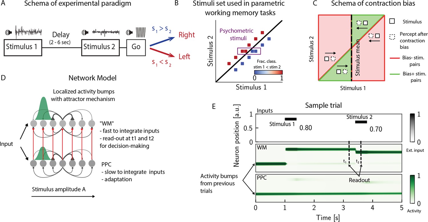
The posterior parietal cortex (PPC) as a slower integrator network.
(A) In any given trial, a pair of stimuli (here, sounds) separated by a variable delay interval is presented to a subject. After the second stimulus, and after a go cue, the subject must decide which of the two sounds is louder by pressing a key (humans) or nose-poking in an appropriate port (rats). (B) The stimulus set. The stimuli are linearly separable, and stimulus pairs are equally distant from the diagonal. Error-free performance corresponds to network dynamics from which it is possible to classify all the stimuli below the diagonal as (shown in blue) and all stimuli above the diagonal as (shown in red). An example of a correct trial can be seen in (E). In order to assay the psychometric threshold, several additional pairs of stimuli are included (purple box), where the distance to the diagonal is systematically changed. The colorbar expresses the fraction classified as . (C) Schematics of contraction bias in delayed comparison tasks. Performance is a function of the difference between the two stimuli, and is impacted by contraction bias, where the base stimulus is perceived as closer to the mean stimulus. This leads to a better/worse (green/red area) performance, depending on whether this ‘attraction’ increases (Bias+) or decreases (Bias-) the discrimination between the base stimulus and the comparison stimulus . (D) Our model is composed of two modules, representing working memory (WM) and sensory history (PPC). Each module is a continuous one-dimensional attractor network. Both networks are identical except for the timescales over which they integrate external inputs; PPC has a significantly longer integration timescale and its neurons are additionally equipped with neuronal adaptation. The neurons in the WM network receive input from those in the PPC through connections (red lines) between neurons coding for the same stimulus. Neurons (gray dots) are arranged according to their preferential firing locations. The excitatory recurrent connections between neurons in each network are a symmetric, decreasing function of their preferential firing locations, whereas the inhibitory connections are uniform (black lines). For simplicity, connections are shown for a single presynaptic neuron (where there is a bump in green). When a sufficient amount of input is given to a network, a bump of activity is formed and sustained in the network when the external input is subsequently removed. This activity in the WM network is read out at two time points: slightly before and after the onset of the second stimulus, and is used to assess performance. (E) The task involves the comparison of two sequentially presented stimuli, separated by a delay interval (top panel, black lines). The WM network integrates and responds to inputs quickly (middle panel), while the PPC network integrates inputs more slowly (bottom panel). As a result, external inputs (corresponding to stimulus 1 and 2) are enough to displace the bump of activity in the WM network, but not in the PPC. Instead, inputs coming from the PPC into the WM network are not sufficient to displace the activity bump, and the trial is consequently classified as correct. In the PPC, instead, the activity bump corresponds to a stimulus shown in previous trials.
Figure 2 with 2 supplements
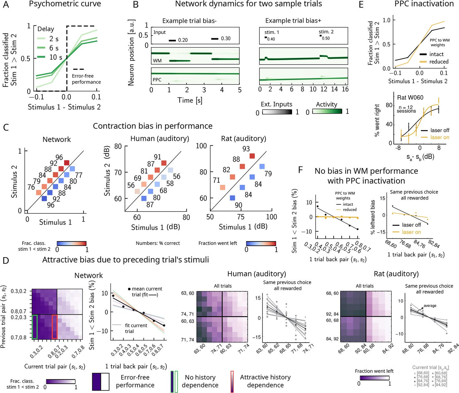
Contraction bias and short-term sensory history effects as a result of posterior parietal cortex (PPC) network activity.
(A) Performance of network model for psychometric stimuli (shades of green) is not error-free (black dashed line). A shorter interstimulus delay interval yields a better performance. (B) Errors occur due to the displacement of the bump representing the first stimulus in the working memory (WM) network. Depending on the direction of this displacement with respect to , this can give rise to trials in which the comparison task becomes harder (easier), leading to negative (positive) biases (top and bottom panels). Top subpanel: stimuli presented to both networks in time. Middle/bottom subpanels show activity of WM and PPC networks (in green). (C) Left: performance is affected by contraction bias – a gradual accumulation of errors for stimuli below (above) the diagonal upon increasing (decreasing) . Colorbar indicates fraction of trials classified as . Middle and right: for comparison, data from the auditory version of the task performed in humans and rats. (D) Panel 1: for each combination of current (x-axis) and previous trial’s stimulus pair (y-axis), fraction of trials classified as (colorbar). Performance is affected by preceding trial’s stimulus pair (modulation along the y-axis). For readability, only some tick-labels are shown. Panel 2: bias, quantifying the (attractive) effect of previous stimulus pairs. Colored lines correspond to linear fits of this bias for each pair of stimuli in the current trial. Black dots correspond to average over all current stimuli, and black line is a linear fit. These history effects are attractive: the smaller the previous stimulus, the higher the probability of classifying the first stimulus of the current trial as small, and vice versa. Panel 3: human auditory trials. Percentage of trials in which humans chose left for each combination of current and previous stimuli; vertical modulation indicates attractive effect of preceding trial. Panel 4: percentage of trials in which humans chose left minus the average value of left choices, as a function of the stimuli of the previous trial, for fixed previous trial response choice and reward. Panels 5 and 6: same as panels 3 and 4 but with rat auditory trials. (E) Top: performance of network, when the weights from the PPC to the WM network are weakened, is improved for psychometric stimuli (yellow curve), relative to the intact network (black curve). Bottom: psychometric curves for rats (only shown for one rat) are closer to error-free during PPC inactivation (yellow) than during control trials (black). (F) Left: the attractive bias due to the effect of the previous trial is present with the default weights (black line), but is eliminated with reduced weights (yellow line). Right: while there is bias induced by previous stimuli in the control experiment (black), this bias is reduced under PPC inactivation (yellow).
© 2018, Springer Nature. Experimental figures in panels (C–F) are reproduced with permission from Figures 2, 3 and Extended Data Figure 1 from Akrami et al., 2018. These panels are not covered by the CC-BY 4.0 licence and further reproduction of this figure would need permission from the copyright holder.
Figure 2—figure supplement 1

Inactivating the inputs from the posterior parietal cortex (PPC) network improves performance, in line with experimental findings.
(A) As in Figure 2C. The performance of the network when the strength of the inputs from the PPC to the working memory (WM) network is weakened (modelling the optogenetic inactivation of the PPC) is dramatically improved, and contraction bias is virtually eliminated. The colorbar corresponds to the fraction classified as . (B) As in Figure 2D. The performance for each stimulus pair in the current trial is improved and no modulation by the previous stimulus pairs can be observed. The colorbar corresponds to the fraction classified as . (C) As in Figure 3B. This improvement of the performance can be traced back to how well the activity bump in the WM network (in purple), before the onset of the second stimulus , tracks the first stimulus (shown in colored dots, each corresponding to a different value of the interstimulus delay interval). Relative to the case in which inputs from the PPC are intact (Figure 3A), it can be seen that the location of the bump tracks the first stimulus with high fidelity. The activity in the PPC (in pink), instead, is identical to that shown previously (Figure 6A), as all the other parameters are kept constant. (D) As in (Figure 2C). The bump location can be quantified not only for the stimulus of the current trial (colored dots, each color corresponding to a given delay interval), but for the four preceding stimuli from the two previous trials (from back to ). With weaker inputs from the PPC (pink), the WM (purple) function of the circuit is disrupted less frequently, and in the majority of the trials, the bump of activity corresponds to the first stimulus .
Figure 2—figure supplement 2
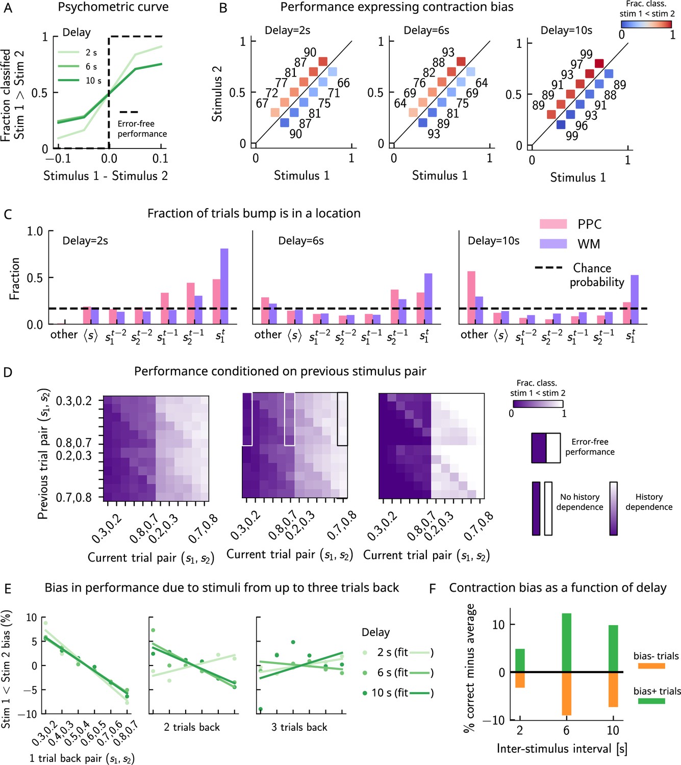
Model predictions for a block design.
(A) As in Figure 2A. Performance of the network model for the psychometric stimuli improves with a short delay interval (light green) and worsens as this delay is increased (dark green). (B) As in Figure 2C. Performance is affected by contraction bias – a gradual accumulation of errors for stimuli below (above) the diagonal upon increasing (decreasing) . As the delay interval increases, the contraction bias is increased which results in reduced performance across all pairs. Colorbar indicates the fraction of trials classified as . (C) As in Figure 3C. The location of the bump that corresponds to the value of occupies a smaller fraction of trials, as the delay interval increases. (D) As in Figure 2D. Performance is affected by the previous stimulus pairs (modulation along the y-axis) and becomes worse as the delay interval is increased. The colorbar corresponds to the fraction classified . (E) As in Figure 3F. Bias, quantifying the (attractive) effect of the previous stimulus pairs, increasing shades of green corresponding to increasing delay intervals. These history effects are attractive: the larger the previous trial stimulus pair, the higher the probability of classifying the first stimulus as large, and vice versa. Middle/right panels: same as the left panel, for stimuli extending two and three trials back. (F) Quantifying contraction bias separately for Bias+ trials (green) and Bias- trials (orange) yields an increasing bias as the interstimulus interval increases.
Figure 3 with 2 supplements
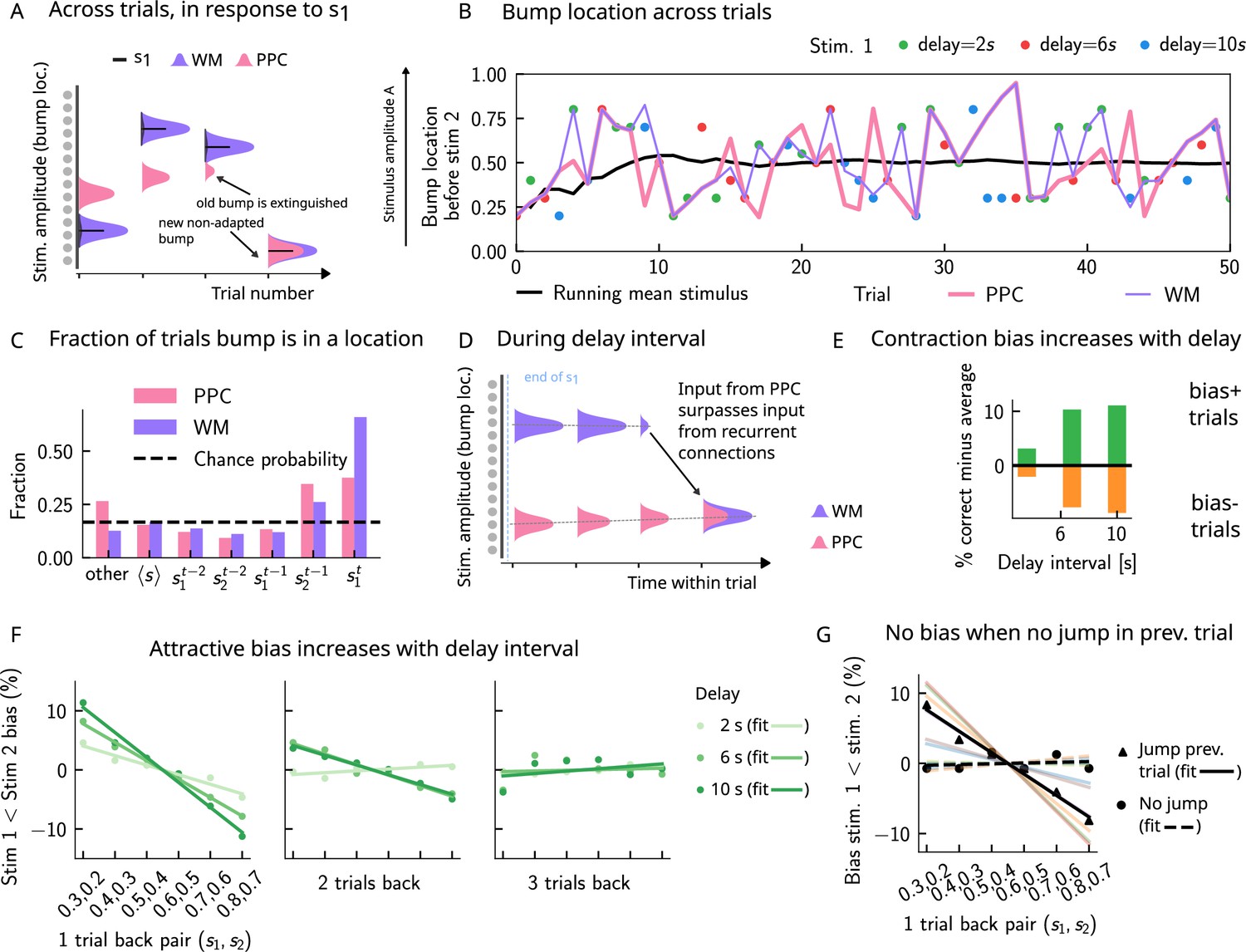
Multiple timescales at the core of short-term sensory history effects.
(A) Schematics of activity bump dynamics in the working memory (WM) vs. posterior parietal cortex (PPC) network. Whereas the WM responds quickly to external inputs, the bump in the PPC drifts slowly and adapts, until it is extinguished and a new bump forms. (B) The location of the activity bump in both the PPC (pink line) and the WM (purple line) networks, immediately before the onset of the second stimulus of each trial. This location corresponds to the amplitude of the stimulus being encoded. The bump in the WM network closely represents the stimulus (shown in colored dots, each color corresponding to a different delay interval). The PPC network, instead, being slower to integrate inputs, displays a continuous drift of the activity bump across a few trials before it jumps to a new stimulus location due to the combined effects of inhibition from incoming inputs and adaptation that extinguishes previous activity. (C) Fraction of trials in which the bump location corresponds to the base stimulus that has been presented () in the current trial, as well as the two preceding trials ( to ). In the WM network, in the majority of trials, the bump coincides with the first stimulus of the current trial . In a smaller fraction of the trials, it corresponds to the previous stimulus due to the input from the PPC. In the PPC network instead, a smaller fraction of trials consist of the activity bump coinciding with the current stimulus . Relative to the WM network, the bump is more likely to coincide with the previous trial’s comparison stimulus (). (D) During the interstimulus delay interval, in the absence of external sensory inputs, the activity bump in the WM network is mainly sustained endogenously by the recurrent inputs. It may, however, be destabilized by the continual integration of inputs from the PPC. (E) As a result, with an increasing delay interval, given that more errors are made, contraction bias increases. Green (orange) bars correspond to the performance in Bias+ (Bias-) regions, relative to the mean performance over all pairs (Figure 1C). (F) Left and middle: longer delay intervals allow for a longer integration times, which in turn lead to a larger frequency of WM disruptions due to previous trials, leading to a larger previous trial attractive biases (2 s vs. 6 s vs. 10 s). Right: weak repulsive effects for larger delays become apparent. Colored dots correspond to the bias computed for different values of the interstimulus delay interval, while colored lines correspond to their linear fits. (G) When neuronal adaptation is at its lowest in the PPC, that is, following a bump jump, the WM bump is maximally susceptible to inputs from the PPC. The attractive bias (toward previous stimuli) is present in trials in which the PPC network underwent a jump in the previous trial (black triangles, with black line a linear fit). Such biases are absent in trials where no jumps occur in the PPC in the previous trial (black dots, with dashed line a linear fit). Colored lines correspond to bias for specific pairs of stimuli in the current trial, regular lines for the jump condition, and dashed for the no jump condition.
Figure 3—figure supplement 1
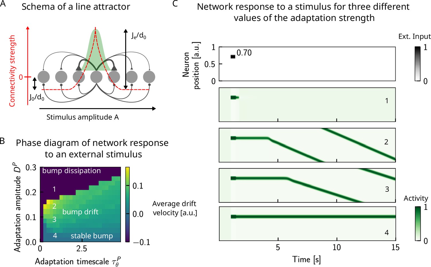
Dynamics of responses in a one-dimensional continuous attractor network in the presence of adaptation.
(A) We study a one-dimensional line attractor in which neurons code for a stimulus feature that varies along a physical dimension, such as amplitude of an auditory stimulus. The connection between pairs of neurons is a decreasing, symmetric function of the distance between their preferred firing locations, allowing for a bump of activity to form and self-sustain when sufficient input is given to the network. However, this self-sustaining activity may be disrupted if neuronal adaptation is present. In particular, drifting dynamics may be observed. (B) Left: phase diagram of the average drift velocity as a function of the adaptation timescale and amplitude . The average drift velocity is simply computed as the distance traveled by the center of the bump in a duration of 50 s. Color codes for the average drift velocity (a.u.). Numbers indicate four points for which sample dynamics are shown in (C). (C) We observe three main phases: in the first, the activity bump is stable when no or little neuronal adaptation is present (point 4). Larger values of neural adaptation induce drift of the activity bump; the average drift velocity increases upon increasing the neural adaptation (points 2 and 3). Finally, increasing it even further leads to the dissipation of the activity bump (point 1). The boundary between the drift and dissipation phases is abrupt. In these simulations, periodic boundary conditions have been used in order to compute the average drift velocity over longer durations.
Figure 3—figure supplement 2

The role of neuronal adaptation in generating short-term history biases.
In order to better understand the network mechanisms that give rise to short-term history effects, we removed neural adaptation in the posterior parietal cortex (PPC) network and assessed the performance in the working memory (WM) network. (A) As in Figure 3B. We track the location of the bump in the PPC (pink) and in WM network (purple) before the onset of the second stimulus (the pink curve cannot be seen as the purple curve goes perfectly on top). In this case, the displacement of the bump of activity is smooth and new sensory stimuli (colored dots) induce only a minimal shift in the location of the bump. This behavior is to be contrasted with the case in which there is adaptation in the PPC network, inducing jumps in the bump location (Figure 3A). An additional effect of no neural adaptation is that the activity in the PPC network completely overrides the activity in the WM network. (B) As in Figure 4A. Marginal distribution of the bump location in both networks (pink for PPC, purple for WM) before the onset of is more peaked than the marginal distribution of the stimuli (gray), as a result of the absence of ‘jumps’. (C) As in Figure 3C. We compute the fraction of times the bump is in a given location, current trial (), four preceding trials ( to ), the running mean stimulus, or all other locations (overlapping sets). In this case, in the majority of the trials, the bump is either at the running mean stimulus or any other location. The fraction of trials in which it is in the position of the four previous stimuli roughly corresponds to chance occurrence (dashed black lines), with only a minor increase for the current stimulus. (D) As in Figure 2D. Left: the network behavior conditioned on the previous trial stimulus pair does not exhibit any previous trial attractive dependence (vertical modulation). Colorbar corresponds to the fraction classified as . Right: this attractive dependence can also be expressed through the bias measure (see main text for how it is computed). Colored lines correspond to current trial pairs, the black dots to the mean over all current trial pairs, and the black line to its linear fit. (E) As in Figure 2C. Although there are no attractive previous trial effects, the performance expresses a very strong contraction bias, and performance is as if the decision boundary is orthogonal to the optimal decision boundary. Color codes for fraction of trials in which a classification is made. (F) Phase diagram with on the x-axis, on the y-axis, and in color, the fraction of trials in which the bump, before the network is stimulated with the second stimulus, is in the vicinity of a target (specified in the title of each panel). White dot corresponds to parameters of the default network (Appendix 1—table 1).
Figure 4 with 1 supplement
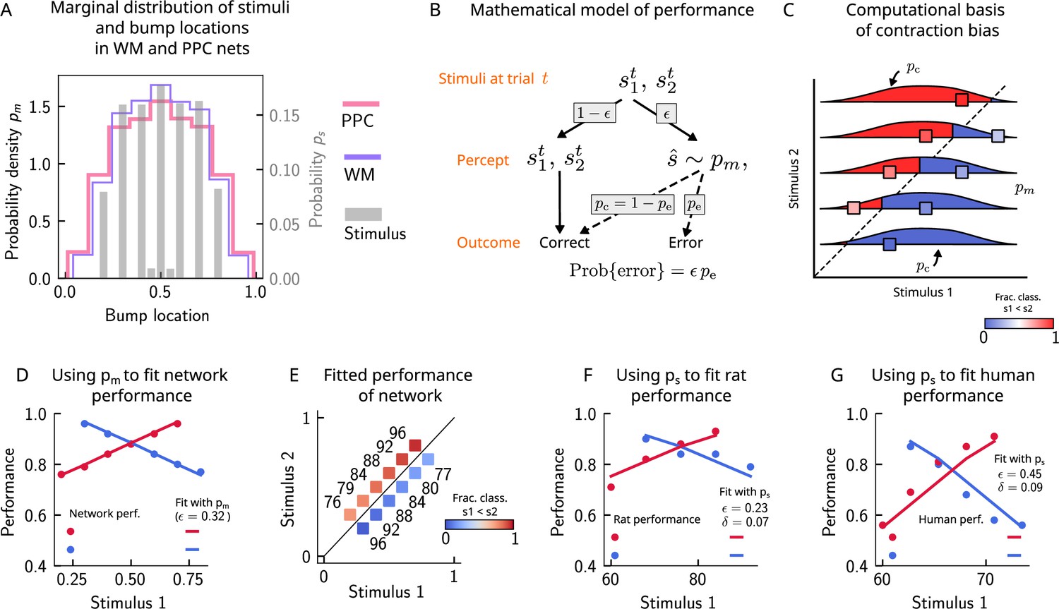
Errors are drawn from the marginal distribution of stimuli, giving rise to contraction bias.
(A) The bump locations in both the working memory (WM) network (in pink) and the posterior parietal cortex (PPC) network (in purple) have identical distributions to that of the input stimulus (marginal over or , shown in gray). (B) A simple mathematical model illustrates how contraction bias emerges as a result of a volatile working memory for . A given trial consists of two stimuli and . We assume that the encoding of the second stimulus is error-free, contrary to the first stimulus that is prone to change, with probability . Furthermore, when does change, it is replaced by another stimulus, (imposed by the input from the PPC in our network model). Therefore, is drawn from the marginal distribution of bump locations in the PPC, which is similar to the marginal stimulus distribution (see panel B), (see also section ‘The probability to make errors is proportional to the cumulative distribution of the stimuli, giving rise to contraction bias‘). Depending on the new location of , the comparison to can either lead to an erroneous choice (Bias-, with probability ) or a correct one (Bias+, with probability ). (C) The distribution of bump locations in PPC (from which replacements are sampled) is overlaid on the stimulus set and repeated for each value of . For pairs below the diagonal, where (blue squares), the trial outcome will be an error if the displaced WM bump ends up above the diagonal (red section of the distribution). The probability to make an error, , equals the integral of over values above the diagonal (red part), which increases as increases. Vice versa, for pairs above the diagonal (, red squares), equals the integral of over values below the diagonal, which increases as decreases. (D) The performance of the attractor network as a function of the first stimulus , in red dots for pairs of stimuli where , and in blue dots for pairs of stimuli where . The solid lines are fits of the performance of the network using Equation 9, with as a free parameter. (E) Numbers correspond to the performance, same as in (D), while colors express the fraction classified as (colorbar), to illustrate the contraction bias. (F) Performance of rats performing the auditory delayed comparison task in Akrami et al., 2018. Dots correspond to the empirical data, while the lines are fits with the statistical model, using the distribution of stimuli. The additional parameter captures the lapse rate. (G) Same as (F), but with humans performing the task. Data in (F) and (G) reproduced with permission from Akrami et al., 2018.
Figure 4—figure supplement 1

The stimulus distribution impacts the pattern of contraction bias.
The model makes different predictions for the performance, depending on the shape of the stimulus distribution. (A) Panel 1: schema of model prediction. Regions shaded in red correspond to the probability of correct comparison for stimulus pairs above the diagonal when replacing with a random value sampled from the marginal distribution with a resampling probability (see Figure 4). Panel 2: prediction of both models for a unimodal symmetric (in this case quasi-uniform) stimulus distribution, statistical model (solid line), and Bayesian model (dashed line). The marginal stimulus distribution is shown in gray bars (to be read with the right y-axis). The value of for which there is equal performance for pairs of stimuli below and above the diagonal is indicated by the vertical dashed line, corresponding to the median of the distribution. Panel 3: for each stimulus pair, fraction of trials classified as (colorbar), for statistical model. Panel 4: same as panel 3, but for Bayesian model of equal average performance (corresponding to a width of the likelihood of (see sections ‘The stimulus distribution impacts the pattern of contraction bias through its cumulative’ and ’Bayesian description of contraction bias’)). (B) Similar to (A), for a negatively skewed distribution. (C) Similar to (A), for a positively skewed distribution. (D) Similar to (A), for a bimodal distribution.
Figure 5
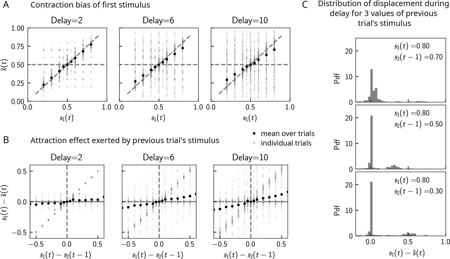
Contraction bias in continuous recall.
(A) We observe contraction bias of the bump of activity after the delay period : the average over trials (black dots) deviates from the identity line (diagonal dashed line) toward the mean of the marginal stimulus distribution (0.5). This effect is stronger as the delay interval is longer (left to right panel). (B) This contraction bias is actually largely due to the effect of the previous trial: the larger the difference between the current trial and the previous trial’s stimulus , the larger is this attractive effect on average. Accordingly with panel (A), this effect is stronger for longer delay intervals (left to right panel). (C) The distribution of the bump displacement during delay period is characterized by two modes: a main one centered around 0, corresponding to correct trials where the working memory (WM) bump is not displaced during the delay interval, and another one centered around , where the bump is displaced during WM (delay interval is randomly selected between 2, 4, and 10 s). We show here this distribution for three values of .
Figure 6
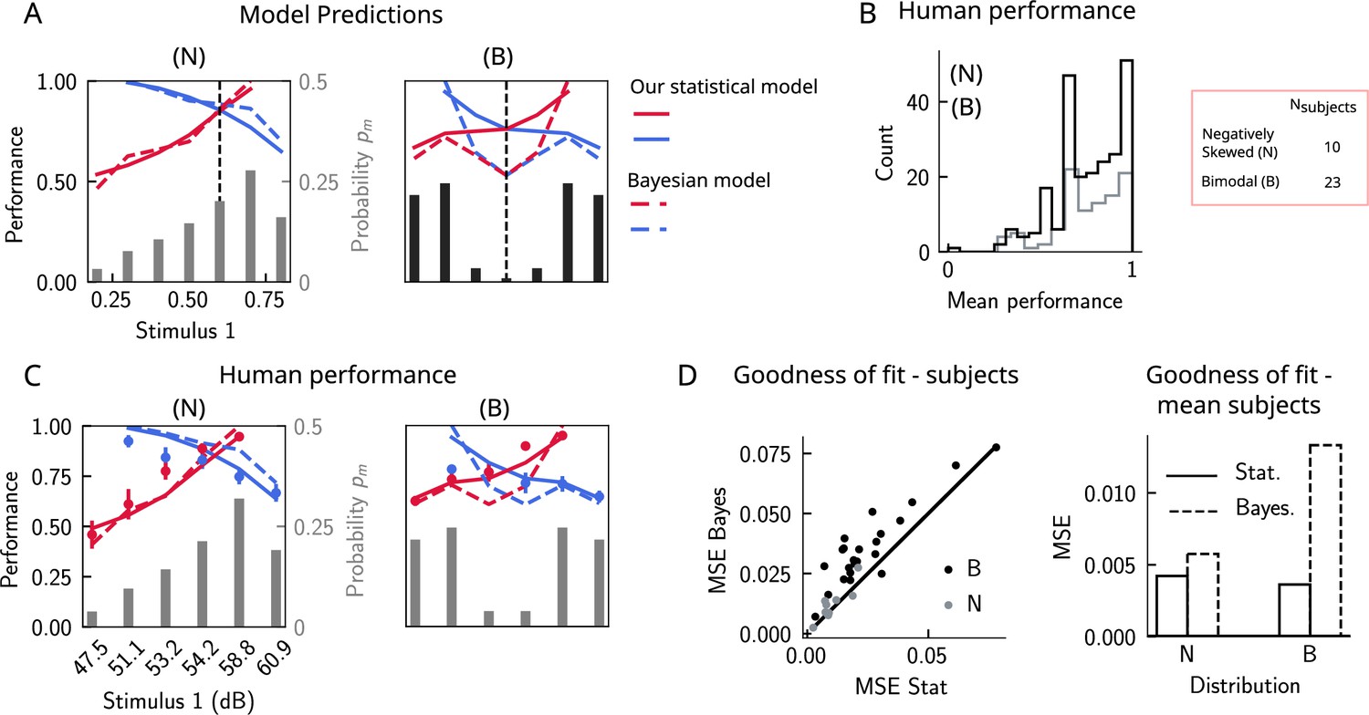
The stimulus distribution impacts the pattern of contraction bias through its cumulative.
(A) Left panel: prediction of performance (left y-axis) of our statistical model (solid lines) and the Bayesian model (dashed lines) for a negatively skewed stimulus distribution (gray bars, to be read with the right y-axis). Blue (red): performance as a function of for pairs of stimuli where (). Vertical dashed line: median of distribution. Right: same as left, but for a bimodal distribution. (B) The distribution of performance across different stimuli pairs and subjects for the negatively skewed (gray) and the bimodal distribution (black). On average, across both distributions, participants performed with an accuracy of 75%. (C) Left: mean performance of human subjects on the negatively skewed distribution (dots, error bars correspond to the standard deviation across different participants). Solid (dashed) lines correspond to fits of the mean performance of subjects with the statistical (Bayesian) model, (). Red (blue): performance as a function of for pairs of stimuli where (), to be read with the left y-axis. The marginal stimulus distribution is shown in gray bars, to be read with the right y-axis. Right: same as left panel, but for the bimodal distribution. Here (). (D) Left: goodness of fit, as expressed by the mean-squared error (MSE) between the empirical curve and the fitted curve (statistical model in the x-axis and the Bayesian model in the y-axis) computed individually for each participant and each distribution. Right: goodness of fit computed for the average performance over participants in each distribution.
Figure 7
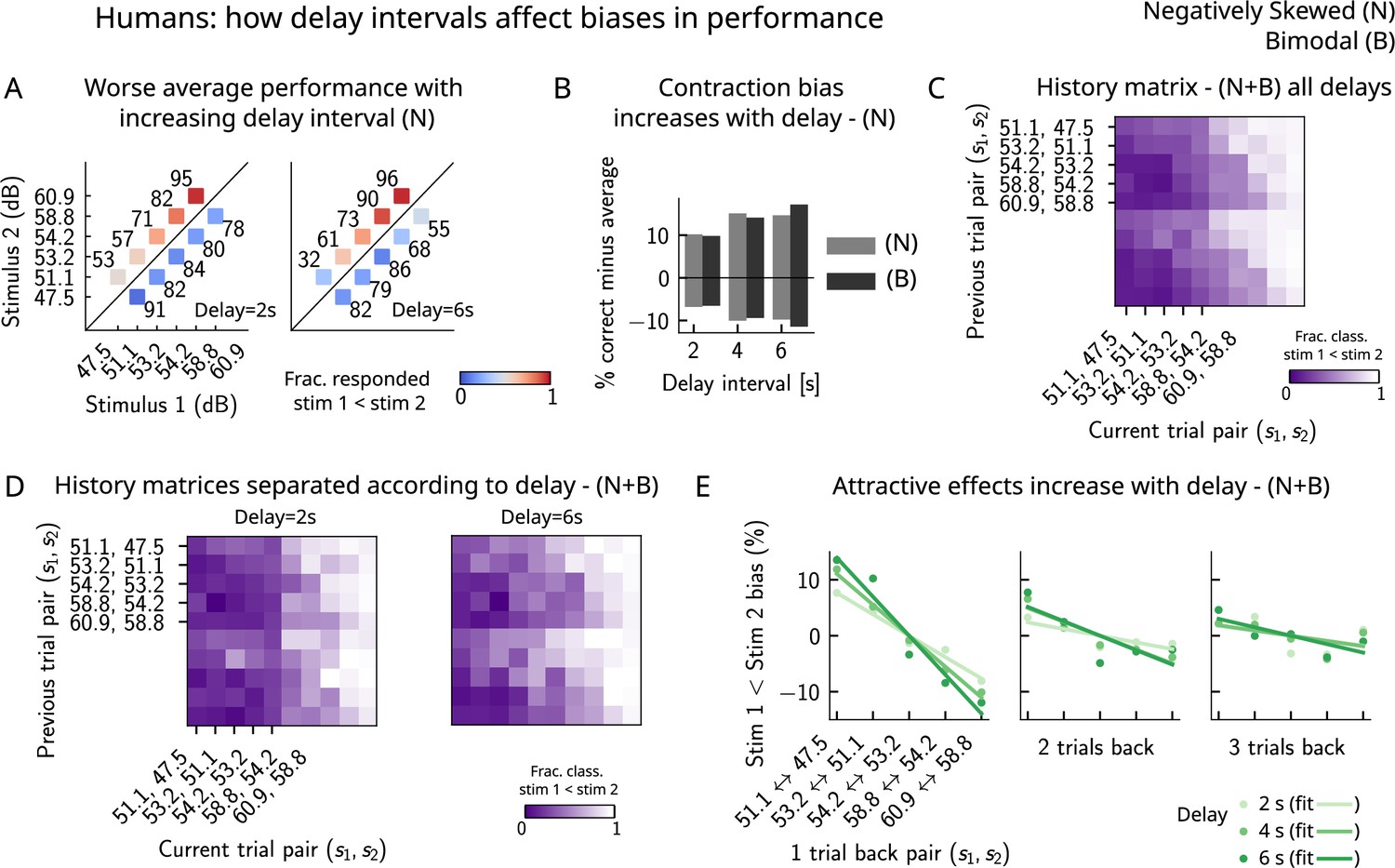
Attractive effects of the previous trials lead to contraction bias in human subjects, both increasing with delay interval.
(A) The performance (in percentage correct, shown in numbers above each stimulus pair) of human subjects is better with lower delay intervals (left, 2 s) than with higher delay intervals (right, 6 s). Colorbar expresses the fraction of trials in which participants responded that . Results are for the negatively skewed stimulus distribution, noted (N). (B) Concurrently, contraction bias on Bias+ and Bias- trials (quantification explained in text) also increases with an increased delay interval for both stimulus distributions (negatively skewed in gray and bimodal in black). (C) History matrix expressing the fraction of trials in which subjects responded (in color) for every pair of current (x-axis) and previous (y-axis) stimuli for negatively skewed and bimodal stimulus distributions (N+B). The one-trial back history effects can be seen through the vertical modulation of the color. Colorbar codes for the fraction of trials in which subjects responded . (D) History matrices (as in [C]) computed for all distributions and separated according to delay intervals (left: 2 s and right: 6 s). (E) Bias, quantifying the (attractive) effect of previous stimulus pairs, for 1–3 trials back in history. The attractive bias computed for all distributions increases with the delay interval separating the two stimuli (light to dark green: increasing delay).
Figure 8
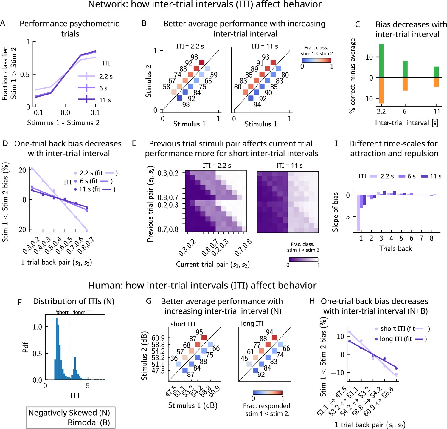
A prolonged intertrial interval (ITI) improves average performance and reduces attractive biases.
Working memory is attracted toward short-term and repelled from long-term sensory history. (A) Performance of the network model for the psychometric stimuli improves with an increasing ITI. Error bars (not visible) correspond to the SEM over different simulations. (B) The network performance (numbers next to stimulus pairs) is on average better for longer ITIs (right panel, ITI = 11 s) compared to shorter ones (left panel, ITI = 2.2 s). Colorbar indicates the fraction of trials classified as . (C) Quantifying contraction bias separately for Bias+ trials (green) and Bias- trials (orange) yields a decreasing bias as the ITI increases. (D) The bias, quantifying the (attractive) effect of the previous trial, decreases with ITI. Darker shades of purple correspond to increasing values of the ITI, with dots corresponding to simulation values and lines to linear fits. (E) Performance is modulated by the previous stimulus pairs (modulation along the y-axis), more for a short ITI (left, ITI = 2.2 s) than for a longer ITI (right, IT I = 11 s). The colorbar corresponds to the fraction classified . (F) The distribution of ITIs in the human experiment is bimodal. We define as having a ‘short’ ITI, those trials where the preceding ITI is shorter than 3 s and conversely for ‘long’ ITI. (G) The human performance for the negatively skewed stimulus distribution is on average worse for shorter ITIs (left panel) compared to longer ones (right panel). Colorbar indicates the fraction of trials subjects responded . (H) The bias, quantifying the (attractive) effect of the previous trial, increases with ITI in human subjects. Darker shades of purple correspond to increasing values of the ITI, with dots corresponding to empirical values and lines to linear fits. (I) Although the stimuli shown up to two trials back yield attractive effects, those further back in history yield repulsive effects, notably when the ITI is larger. Such repulsive effects extend to up to six trials back.
Figure 9 with 1 supplement
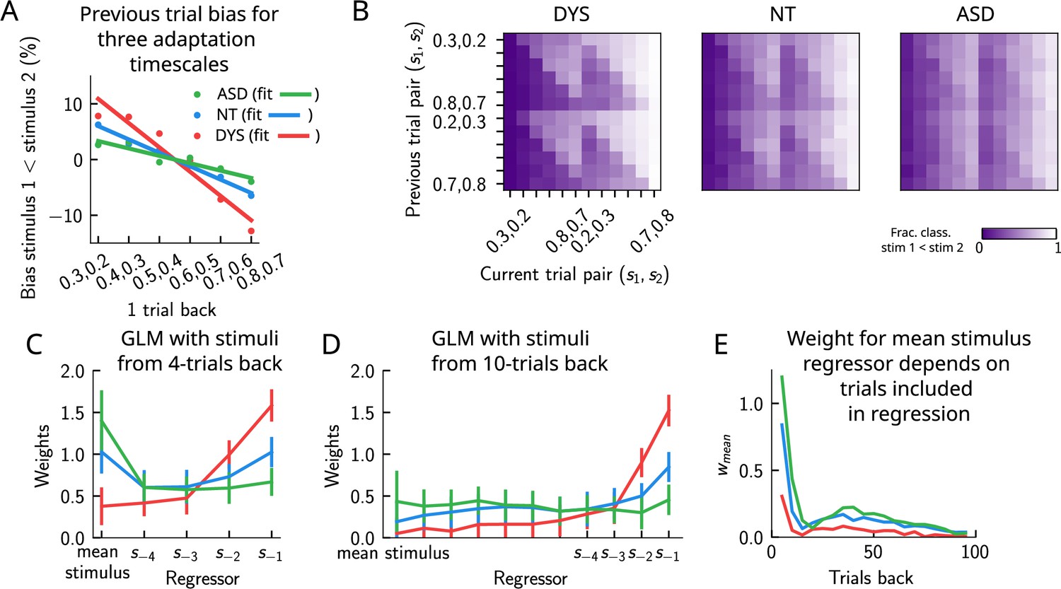
Apparent tradeoff between short- and long-term biases controlled by the timescale of neural adaptation.
(A) The bias exerted on the current trial by the previous trial (see main text for how it is computed) for three values of the adaptation timescale that mimic similar behavior to the three cohorts of subjects. (B) As in Figure 2D, for three different values of adaptation timescale. The colorbar corresponds to the fraction classified . (C) Generalized linear model (GLM) weights corresponding to the three values of the adaptation parameter marked in Figure 9—figure supplement 1A, including up to four trials back. In a GLM variant incorporating a small number of past trials as regressors, the model yields a high weight for the running mean stimulus regressor. Error bars correspond to the standard deviation across different simulations. (D) Same as in (C), but including regressors corresponding to the past 10 trials as well as the running mean stimulus. With a larger number of regressors extending into the past, the model yields a small weight for the running mean stimulus regressor. Error bars correspond to the standard deviation across different simulations. (E) The weight of the running mean stimulus regressor as a function of extending the number of past trial regressors decays upon increasing the number of previous trial stimulus regressors.
Figure 9—figure supplement 1
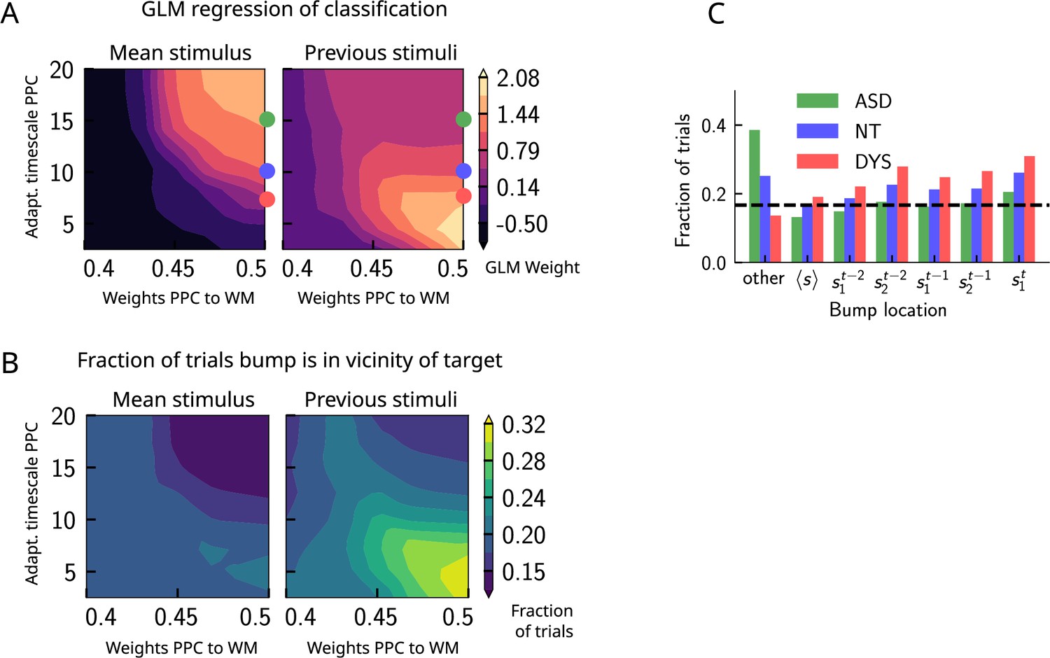
Apparent tradeoff between short- and long-term biases controlled by the timescale of neural adaptation.
(A) Left: generalized linear model (GLM) weight associated with the regressor corresponding to the mean stimulus across trials (value indicated by colorbar) as a function of the strength of the weights from the posterior parietal cortex (PPC) to the working memory (WM) network (x-axis), and the adaptation timescale in the PPC (y-axis). Right: Same as the left panel, but displaying the GLM weight associated with the regressor corresponding to the previous trial’s stimulus. These two panels indicate that the adaptation timescale seemingly exerts a tradeoff between the two biases: while decreasing it increases short-term sensory history biases, and increasing it increases long-term sensory history biases. The values of the adaptation parameter marked by the three colored dots (in red, blue, and green) can mimic behaviors similar to dyslexic, neurotypical, and autistic spectrum subjects (see also Figure 9). (B) Left: phase diagram of the fraction of trials in which the activity bump at the end of the delay interval is in the location of the running mean stimulus as a function of the strength of the weights from the PPC to the WM network (x-axis), and the adaptation timescale in the PPC (y-axis). Right: same as (left), but for the location of any of the two stimuli presented in the previous trial. (C) The fraction of trials in which the activity bump at the end of the delay interval corresponds to different locations shown in the x-axis for three different values of the adaptation timescale parameter corresponding to qualitatively similar to dyslexic, neurotypical, and autistic spectrum subjects, shown in colors.
Tables
Appendix 1—table 1
Simulation parameters, when not explicitly mentioned.
Used to produce Figures 1—5 and 8, Figure 2—figure supplements 1 and 2, and Figure 3—figure supplement 2.
| Parameter | Symbol | Default value |
|---|---|---|
| Number of neurons | 2000 | |
| Neuronal gain | 5 | |
| Range of excitatory interactions (in units of stimulus space length) | 0.02 | |
| Strength of inhibitory weights | 0.2 | |
| Strength of excitatory weights | 1 | |
| Timescale of neuronal integration in WM net (s) | 0.01 | |
| Timescale of neuronal integration in PPC (s) | 0.5 | |
| Timescale of neuronal adaptation in PPC (s) | 7.5 | |
| Amplitude of adaptation current in PPC | 0.3 | |
| Amplitude of external inputs | 1 | |
| Strength of weights from PPC to WM net | 0.5 | |
| Duration of stimuli (s) | 0.4 | |
| Delay interval (s) | [2, 6, 10] | |
| Intertrial interval (s) | 6 | |
| Width of box stimulus (in units of stimulus space length) | 0.05 |
-
WM, working memory; PPC, posterior parietal cortex.
Appendix 1—table 2
Simulation parameters (Figure 3—figure supplement 1).
| Parameter | Symbol | Default value |
|---|---|---|
| Number of neurons | 1000 | |
| Neuronal gain | 5 | |
| Range of excitatory interactions (in units of stimulus space length) | 0.02 | |
| Strength of inhibitory weights | 0.2 | |
| Strength of excitatory weights | 1 | |
| Timescale of neuronal integration (s) | 0.01 | |
| Amplitude of external inputs | 1 | |
| Duration of stimuli (s) | 0.4 | |
| Width of box stimulus (in units of stimulus space length) | 0.05 |
Appendix 1—table 3
Simulation parameters (Figure 9 and Figure 9—figure supplement 1).
Other parameters as in Table 1Appendix 1—table 1.
| Parameter | Symbol | Default value |
|---|---|---|
| Timescale of neuronal adaptation in PPC (s) | 7.5 (DYS), 10 (NT), 15 (ASD) | |
| Amplitude of adaptation in PPC | 0.2 | |
| Delay interval (s) | [2, 6, 10] | |
| Intertrial interval (s) | 2.2 |
-
ASD, autistic spectrum; DYS, dyslexic; NT, neurotypical; PPC, posterior parietal cortex.
Additional files
Download links
A two-part list of links to download the article, or parts of the article, in various formats.
Downloads (link to download the article as PDF)
Open citations (links to open the citations from this article in various online reference manager services)
Cite this article (links to download the citations from this article in formats compatible with various reference manager tools)
Unifying network model links recency and central tendency biases in working memory
eLife 12:RP86725.
https://doi.org/10.7554/eLife.86725.3


